
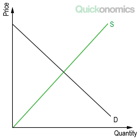
Updated Oct 13, 2020 Producer Surplus describes the difference between the amount of money at which sellers are willing and able to sell a good or service (i.e. willingness to sell) and the amount they actually end up receiving (i.e. the market price). Every seller has an individual willingness to sell. That means, if the market price is below that amount, they will not sell their good or service. On the other hand, as long as the market price is above or equal to their individual willingness to sell, they will accept the price, sell their products, and thereby earn a producer surplus. In the following paragraphs, we will take a closer look at how to calculate producer surplus. To do this, we will follow a simple 4-step process: (1) draw the supply and demand curves, (2) find the market price, (3) connect the price axis and the market equilibrium, and (4) calculate the area of the lower triangle. In addition to that, you can also find a step-by-step tutorial in the video below. The calculation of producer surplus works pretty much like the calculation of consumer surplus. We start with a supply and demand diagram. As you can see in the diagram above, the x-axis shows quantity while the y-axis shows price (in USD). Hint: If you are not familiar with the concept of supply and demand at this point, please make sure to read our article on the law of supply and demand first. We will walk through the process with the help of a simple example. Let’s take the market for burgers. Before we can calculate a supply and demand diagram for this market, we need to know the supply and demand functions first. We will look at how to calculate them in different posts (how to calculate a demand function / how to calculate a supply function), for now, let’s just assume that the demand function is QD = -166.7x + 1000 and the supply function is QS=166.7x. We use linear functions here (y = ax + b) for the sake of simplicity. However, please note that supply and demand functions do not necessarily have to be linear. With that being said, we can now use the two functions to draw our supply and demand curves.1) Draw the Supply and Demand Curves
2) Find the Market Equilibrium
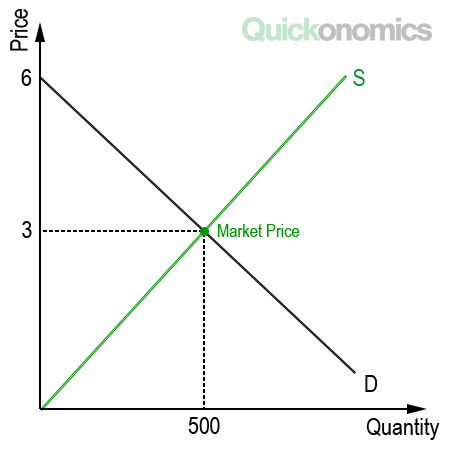
Once we have our supply and demand diagram, we can find the market equilibrium. It is located at the intersection of the supply and the demand curve. That means, to calculate it we have to first set the demand function equal to the supply function and solve for x. This gives us the equilibrium price. Then we can plug this number back into the demand function and solve for Q to get the equilibrium quantity.
Using our example, the equilibrium condition can be calculated as -166.7x + 1000 = 166.7x. In this equation, x equals 3. That means when the price is USD 3.00, the market is in equilibrium. Now, if we plug this number back into the supply function (QS = 166.7*3), we find that the equilibrium quantity is 500 burgers. In other words, when the market is in equilibrium, 500 burgers can be sold at a price of USD 3.00 each.
3) Connect the Price Axis and the Market Price

Once we have calculated the market price and quantity, we can add these numbers to the supply and demand diagram. As you can see, the market price is generally not the lowest possible price at which the good or service could be sold. This means, there are at least some sellers who would have been willing to sell the product at a lower price than the actual market price. These sellers can now earn a producer surplus, equal to the market price minus their individual willingness to sell. We can illustrate this by drawing a horizontal line between the y-axis and the market equilibrium (i.e. the intersection of S and D).
If we draw this horizontal line for our example, we see that it intersects the y-axis at a price of USD 3.00. As you can see in the illustration above, the line divides the area between the supply and the demand curve into two triangles. One triangle above the USD 3.00 line and another one below. The area of the lower triangle represents the sum of all individual producer surpluses, which equals total producer surplus.
4) Calculate the Area of the Lower Triangle
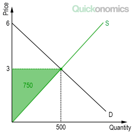
To calculate the area of the lower triangle, we need to multiply its base with the height and divide the result by two (a = [b*h]/2). Please note that this formula only works with linear supply curves. Other types of supply curves require a more complex formula to calculate the area between two curves (see Wolfram|Alpha for more information).
If we apply this to our example, we can easily calculate the area of the lower triangle. We know that the base of the triangle is 500 and its height is 3.00. Thus, we can use the following equation: (500*3)/2 = 750.00. Thus, the total producer surplus in our burger market is equal to USD 750.00.
Summary
Producer Surplus describes the difference between the amount of money at which sellers are willing and able to sell a good or service (i.e. willingness to sell) and the amount they actually end up receiving (i.e. the market price). Calculating producer surplus follows a 4-step process: (1) draw the supply and demand curves, (2) find the market equilibrium, (3) connect the price axis and the market price, and (4) calculate the area of the lower triangle.