How to Calculate Consumer Surplus

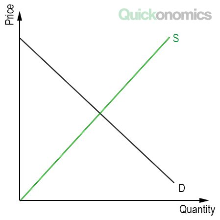
Updated Oct 13, 2020

Consumer Surplus is defined as the difference between the amount of money consumers are willing and able to pay for a good or service (i.e. willingness to pay) and the amount they actually end up paying (i.e. the market price). Every consumer has an individual willingness to pay for a specific product. Thus, if the market price is above that amount, they will not buy that particular good or service. However, as long as the market price is below or equal to their individual willingness to pay, they will purchase the product to satisfy their needs.

So how can we calculate consumer surplus, given its individual nature? Well, that’s actually not as complicated as it may sound. In fact, calculating consumer surplus follows a simple 4-step process: (1) draw the supply and demand curves, (2) find the market price, (3) connect the price axis and the market price, and (4) calculate the area of the upper triangle.

1) Draw the Supply and Demand Curves

The easiest way to calculate consumer surplus is with the help of a supply and demand diagram. The diagram above has quantity on the x-axis and price (in USD) on the y-axis. Please note that it is critical to understand the relationship between supply and demand first in order to fully comprehend the concept of consumer surplus. So if you are not familiar with supply and demand yet, make sure to read our article on the law of supply and demand first.

Once again, we will use a simple example to walk through the process. Let’s look at an imaginary burger restaurant called Super Burger. If we want to draw the supply and demand diagram for this restaurant, we need to know the corresponding functions first. You can learn how to calculate linear demand functions in a different post. For now, let’s just say the demand function is Q_D = -166.7x + 1000, and the supply function is Q_S=166.7x. Note that we are using linear functions (y = ax + b) for the sake of simplicity. However, be aware that not all supply and demand functions are linear. We can now use the two functions to draw the supply and demand curves.

2) Find the Market Price

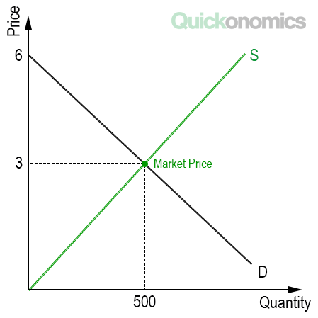
Now that we have drawn the supply and demand curves, we can locate the market price (i.e. the equilibrium price). As we know (according to the law of supply and demand), the market price is located at the intersection of the supply and the demand curve (i.e. supply function = demand function). Thus, to calculate the market price we first need to solve this equation for the equilibrium quantity. Then we can find the corresponding price by plugging the result back into the supply (or demand) function.

In our example, the equilibrium quantity can be calculated as -166.7x + 1000 = 166.7x. If we solve this equation for x, we find that x=3.00 USD. That means, in the market equilibrium, Super Burger can sell its burgers at a price of 3.00 USD. If we plug this back into the supply function (Q_S=166.7*3) we find that the equilibrium quantity is 500 burgers. In other words, Super Burger can sell a total of 500 burgers at a market price of USD 3.00 per burger.

3) Connect the Price Axis and the Market Price

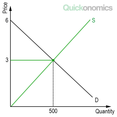
Now that we have calculated the market price and quantity, we can take another look at the supply and demand diagram. As you can see, the market price is usually not the highest possible price at which the product could be sold. That means, there are usually at least consumers who would have been willing to buy the good or service at a higher price than the actual market price. These consumers now enjoy a consumer surplus of their individual willingness to pay minus the market price. To illustrate this, we can draw a horizontal line between the y-axis and the market equilibrium (i.e. the intersection of the supply (S) and demand curve (D)). 

In our example, this line intersects the y-axis at USD 3.00. This creates two triangles, one above the USD 3.00 line and another one below the line. The area of the upper triangle represents the sum of all individual consumer surpluses, which is equal to the total consumer surplus. We will look at how to calculate it in the next step.

4) Calculate the Area of the Upper Triangle

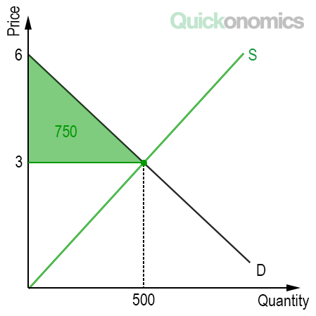
To calculate the area of the upper triangle, we can multiply its base with the height and then divide the result by two (area = [b*h]/2). This holds true as long as the demand curve is linear. If that’s not the case we have to use a more complex formula to calculate the area under the curve (note: Wolfram|Alpha has a useful widget to help you with that).

Going back to our example, we can calculate the area of the upper triangle as follows: The base of the triangle is 500 and the height is 3.00. If we plug this into the formula we get (500*3)/2 = 750.00. That means the total consumer surplus is USD 750.00.

In a Nutshell

Consumer Surplus is defined as the difference between the amount of money consumers are willing and able to pay for a good or service (i.e. willingness to pay) and the amount they actually end up paying (i.e. the market price. To calculate consumer surplus we can follow a simple 4-step process: (1) draw the supply and demand curves, (2) find the market price, (3) connect the price axis and the market price, and (4) calculate the area of the upper triangle.