
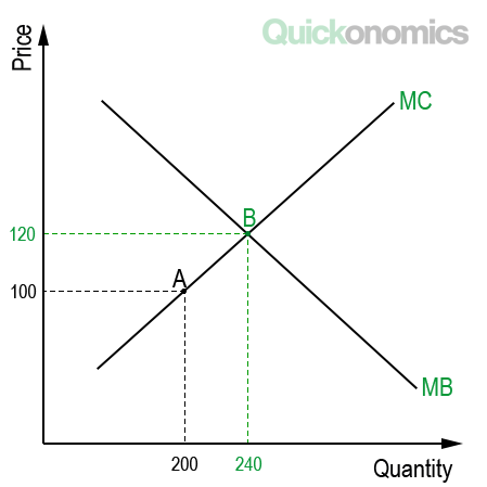
Updated Jun 26, 2020 Economics is all about efficiency. Most economic issues arise because of scarce resources. Starting from there, we often have to find ways to use, produce, and distribute those resources in the best possible way (i.e., efficient). However, depending on the issue we are looking at, there may be different factors that define whether a situation is considered efficient or not. In other words, there are several different types of economic efficiency. We will look at five of them in more detail below: allocative, productive, dynamic, social, and X-efficiency. Allocative efficiency occurs when all goods and services within an economy are distributed according to consumer preferences. In this scenario, price always equals the marginal cost of production. The reason for this is that the price consumers are willing to pay for a product or service reflects the marginal utility they get from consuming the product. Hence, the optimal outcome is achieved when the marginal cost (MC) equals marginal benefit (MB). This is illustrated in the graph below. The optimal outcome in the illustration is marked by point B (i.e., 240 units of output for USD 120). This is at the intersection of the marginal cost curve and the marginal benefit curve. By contrast, point A does not represent an allocatively efficient outcome, because the marginal cost of production does not equal marginal benefit at this point. Allocative efficiency can be found in perfectly competitive markets because firms in those markets don’t have enough market power to increase prices. To survive, they have to produce what society values most, at the prices, consumers are willing to pay. By contrast, Monopolies are said to produce allocatively inefficient levels of output, simply because they have enough market power to affect prices and reduce consumer surplus by engaging in price discrimination.Allocative Efficiency
Productive Efficiency
Productive efficiency occurs when the optimal combination of inputs results in the maximum amount of output at minimal costs. That is the case when firms operate at the lowest point of their average total cost curve (i.e., where marginal costs equal average costs). A productively efficient economy always produces on its production possibility frontier. That means that the economy can’t produce more of one good or service without reducing the production of another one.
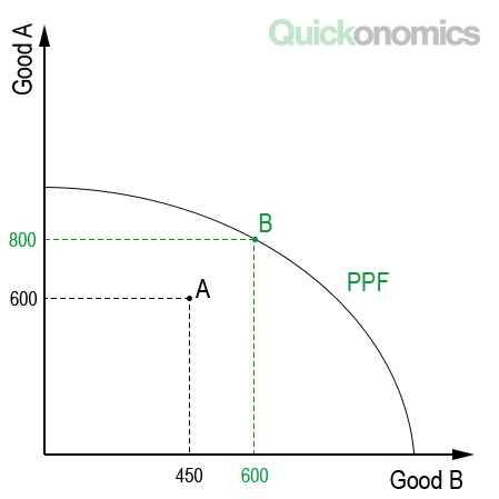
The illustration above shows the production possibility frontier (PPF) for two goods (A and B). If an economy produces 600 units of good A and 450 units of good B, it is not working at full capacity. More units of both goods could be produced without reducing the production of the other good. Thus, we have productive inefficiency. However, if the same economy produces 800 units of good A and 600 units of good B, it produces on the PPF, which is productively efficient. Please note that all points on the PPF represent a productively efficient outcome.
Productive efficiency requires all firms to use the least costly factors of production (e.g., land, labor), the best processes, and the most advanced technology available. Also, wastage during production has to be reduced to a minimum, and possible economies of scale have to be realized. If those conditions are met, it won’t be possible for the firms to produce more goods or services without more inputs.
Keep in mind that productive efficiency does not necessarily have to entail allocative efficiency. For example, if society does not need 800 units of good A and 600 units of good B, the illustration above does not describe an allocatively efficient outcome even though it is productively efficient.
Dynamic Efficiency
Dynamic efficiency occurs over time, as innovation and new technologies reduce production costs. In essence, it describes the productive efficiency of an economy (or firm) over time. We speak of dynamic efficiency when an economy or firm manages to shift its average cost curve (short and long run) down over time. This can be boosted by research and development, investments in human capital, or an increase in competition within the market. The graph below illustrates dynamic efficiency.
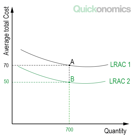
As we can see, the first long-run average cost curve (LRAC 1) lies above the second long-run average cost curve (LRAC 2). In many cases, this is what happens over time, as innovation helps to improve products and processes and thus reduce costs. Lower average costs allow firms to sell at a lower price, which is why point A and the entire LRAC 1 shifts down to point B (and LRAC 2) over time.
An economy with a high dynamic efficiency generally offers more choices of high-quality goods for consumers. This is because invention and innovation not only result in better processes and lower cost but also higher quality goods and services for consumers.
Social Efficiency
Social Efficiency occurs when goods and services are optimally distributed within an economy, also taking externalities into account. This is the case when the marginal social cost of production equals social benefit. This relationship can be illustrated as follows.
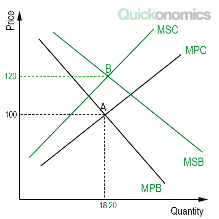
The graph shows two sets of curves. The intersection of the marginal private cost curve (MPC) and the marginal private benefit curve (MPB) represents an allocatively efficient outcome (point A). However, if we take externalities into account as well, we have to look at the intersection of the marginal social cost curve (MSC) and the marginal social benefit curve (MSB) instead. Hence, the socially efficient outcome is not reached at point A (18 units for USD 100) but shifts up to point B (20 units for USD 120).
In a socially efficient economy, overall social welfare is maximized. However, in most cases, this requires some form of taxation. In a free market, both consumers and producers don’t take externalities into account. As a result, taxes (or subsidies) are required to internalize the externalities and reach a socially efficient outcome (see also Positive and Negative Externalities).
X-efficiency
X-efficiency occurs when a firm has an incentive to produce maximum output with a given amount of input. Hence, it is quite similar to productive efficiency. The main difference between the two is that X-efficiency depends on management incentives, whereas productive efficiency depends on processes and technology.
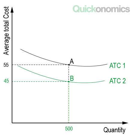
The illustration above shows an inefficient average total cost curve (ATC 1) and an efficient total cost curve (ATC 2) of a firm. This looks quite similar to the illustration of dynamic efficiency. However, in this case, the shift from point A to point B does not depend on innovation but only on management incentives. That means the firm can shift its average total costs to ATC 2 from the beginning. However, it does not have any incentives to do so.
We are most likely to encounter X-efficiency in highly competitive markets. In those situations, the management has to produce as much output as possible (at the lowest possible cost) to remain competitive. By contrast, in a monopoly, we will usually see a loss of X-efficiency, because the monopolist can increase profits by not maximizing output.
In a Nutshell
Most economic issues arise because of scarce resources. Hence, it is critical to use, produce, and efficiently distribute those resources. There are several different types of economic efficiency. The five most relevant ones are allocative, productive, dynamic, social, and X-efficiency. Allocative efficiency occurs when goods and services are distributed according to consumer preferences. Productive efficiency is a situation where the optimal combination of inputs results in the maximum amount of output. Dynamic efficiency occurs over time, as innovation reduces production costs. Social Efficiency happens when goods and services are optimally distributed, also taking externalities into account. And last but not least, X-efficiency occurs when a firm has an incentive to produce maximum output with a given amount of input.